Preparing the data for analysis

Before beginning our analysis, it is critical that we first examine and clean the dataset, to make working with it a more efficient process. We will fixing data types, handle missing values, and dropping columns and rows while exploring the Stanford Open Policing Project dataset.

Stanford Open Policing Project dataset

Examining the dataset

We’ll be analyzing a dataset of traffic stops in Rhode Island that was collected by the Stanford Open Policing Project.

Before beginning our analysis, it’s important that we familiarize yourself with the dataset. We read the dataset into pandas, examine the first few rows, and then count the number of missing values.

Libraries

import pandas as pd
import matplotlib.pyplot as plt
from pandas.api.types import CategoricalDtype

# Read 'police.csv' into a DataFrame named ri
ri = pd.read_csv("../datasets/police.csv")

# Examine the head of the DataFrame
display(ri.head())

# Count the number of missing values in each column
ri.isnull().sum()

	state	stop_date	stop_time	county_name	driver_gender	driver_race	violation_raw	violation	search_conducted	search_type	stop_outcome	is_arrested	stop_duration	drugs_related_stop	district
0	RI	2005-01-04	12:55	NaN	M	White	Equipment/Inspection Violation	Equipment	False	NaN	Citation	False	0-15 Min	False	Zone X4
1	RI	2005-01-23	23:15	NaN	M	White	Speeding	Speeding	False	NaN	Citation	False	0-15 Min	False	Zone K3
2	RI	2005-02-17	04:15	NaN	M	White	Speeding	Speeding	False	NaN	Citation	False	0-15 Min	False	Zone X4
3	RI	2005-02-20	17:15	NaN	M	White	Call for Service	Other	False	NaN	Arrest Driver	True	16-30 Min	False	Zone X1
4	RI	2005-02-24	01:20	NaN	F	White	Speeding	Speeding	False	NaN	Citation	False	0-15 Min	False	Zone X3

state                     0
stop_date                 0
stop_time                 0
county_name           91741
driver_gender          5205
driver_race            5202
violation_raw          5202
violation              5202
search_conducted          0
search_type           88434
stop_outcome           5202
is_arrested            5202
stop_duration          5202
drugs_related_stop        0
district                  0
dtype: int64

It looks like most of the columns have at least some missing values. We’ll figure out how to handle these values in the next.

Dropping columns

We’ll drop the county_name column because it only contains missing values, and we’ll drop the state column because all of the traffic stops took place in one state (Rhode Island).

# Examine the shape of the DataFrame
print(ri.shape)

# Drop the 'county_name' and 'state' columns
ri.drop(["county_name", "state"], axis='columns', inplace=True)

# Examine the shape of the DataFrame (again)
print(ri.shape)

(91741, 15)
(91741, 13)

We’ll continue to remove unnecessary data from the DataFrame

### Dropping rows

the driver_gender column will be critical to many of our analyses. Because only a small fraction of rows are missing driver_gender, we’ll drop those rows from the dataset.

# Count the number of missing values in each column
display(ri.isnull().sum())

# Drop all rows that are missing 'driver_gender'
ri.dropna(subset=["driver_gender"], inplace=True)

# Count the number of missing values in each column (again)
display(ri.isnull().sum())

# Examine the shape of the DataFrame
ri.shape

stop_date                 0
stop_time                 0
driver_gender          5205
driver_race            5202
violation_raw          5202
violation              5202
search_conducted          0
search_type           88434
stop_outcome           5202
is_arrested            5202
stop_duration          5202
drugs_related_stop        0
district                  0
dtype: int64

stop_date                 0
stop_time                 0
driver_gender             0
driver_race               0
violation_raw             0
violation                 0
search_conducted          0
search_type           83229
stop_outcome              0
is_arrested               0
stop_duration             0
drugs_related_stop        0
district                  0
dtype: int64

(86536, 13)

We dropped around 5,000 rows, which is a small fraction of the dataset, and now only one column remains with any missing values.

Using proper data types

Finding an incorrect data type

ri.dtypes

stop_date             object
stop_time             object
driver_gender         object
driver_race           object
violation_raw         object
violation             object
search_conducted        bool
search_type           object
stop_outcome          object
is_arrested           object
stop_duration         object
drugs_related_stop      bool
district              object
dtype: object

stop_date: should be datetime
stop_time: should be datetime
driver_gender: should be category
driver_race: should be category
violation_raw: should be category
violation: should be category
district: should be category
is_arrested: should be bool

We’ll fix the data type of the is_arrested column

# Examine the head of the 'is_arrested' column
display(ri.is_arrested.head())

# Change the data type of 'is_arrested' to 'bool'
ri['is_arrested'] = ri.is_arrested.astype('bool')

# Check the data type of 'is_arrested' 
ri.is_arrested.dtype

0    False
1    False
2    False
3     True
4    False
Name: is_arrested, dtype: object

dtype('bool')

Creating a DatetimeIndex

Combining object columns

Currently, the date and time of each traffic stop are stored in separate object columns: stop_date and stop_time. We’ll combine these two columns into a single column, and then convert it to datetime format.

ri['stop_date_time'] = pd.to_datetime(ri.stop_date.str.replace("/", "-").str.cat(ri.stop_time, sep=" "))
ri.dtypes

stop_date                     object
stop_time                     object
driver_gender                 object
driver_race                   object
violation_raw                 object
violation                     object
search_conducted                bool
search_type                   object
stop_outcome                  object
is_arrested                     bool
stop_duration                 object
drugs_related_stop              bool
district                      object
stop_date_time        datetime64[ns]
dtype: object

Setting the index

# Set 'stop_datetime' as the index
ri.set_index("stop_date_time", inplace=True)

# Examine the index
display(ri.index)

# Examine the columns
ri.columns

DatetimeIndex(['2005-01-04 12:55:00', '2005-01-23 23:15:00',
               '2005-02-17 04:15:00', '2005-02-20 17:15:00',
               '2005-02-24 01:20:00', '2005-03-14 10:00:00',
               '2005-03-29 21:55:00', '2005-04-04 21:25:00',
               '2005-07-14 11:20:00', '2005-07-14 19:55:00',
               ...
               '2015-12-31 13:23:00', '2015-12-31 18:59:00',
               '2015-12-31 19:13:00', '2015-12-31 20:20:00',
               '2015-12-31 20:50:00', '2015-12-31 21:21:00',
               '2015-12-31 21:59:00', '2015-12-31 22:04:00',
               '2015-12-31 22:09:00', '2015-12-31 22:47:00'],
              dtype='datetime64[ns]', name='stop_date_time', length=86536, freq=None)

Index(['stop_date', 'stop_time', 'driver_gender', 'driver_race',
       'violation_raw', 'violation', 'search_conducted', 'search_type',
       'stop_outcome', 'is_arrested', 'stop_duration', 'drugs_related_stop',
       'district'],
      dtype='object')

Exploring the relationship between gender and policing

Does the gender of a driver have an impact on police behavior during a traffic stop? We will explore that question while doing filtering, grouping, method chaining, Boolean math, string methods, and more!

Do the genders commit different violations?

Examining traffic violations

Before comparing the violations being committed by each gender, we should examine the violations committed by all drivers to get a baseline understanding of the data.

We’ll count the unique values in the violation column, and then separately express those counts as proportions.

# Count the unique values in 'violation'
display(ri.violation.value_counts())

# Express the counts as proportions
ri.violation.value_counts(normalize=True)

Speeding               48423
Moving violation       16224
Equipment              10921
Other                   4409
Registration/plates     3703
Seat belt               2856
Name: violation, dtype: int64

Speeding               0.559571
Moving violation       0.187483
Equipment              0.126202
Other                  0.050950
Registration/plates    0.042791
Seat belt              0.033004
Name: violation, dtype: float64

More than half of all violations are for speeding, followed by other moving violations and equipment violations.

Comparing violations by gender

The question we’re trying to answer is whether male and female drivers tend to commit different types of traffic violations.

We’ll first create a DataFrame for each gender, and then analyze the violations in each DataFrame separately.

# Create a DataFrame of female drivers
female = ri[ri.driver_gender=="F"]

# Create a DataFrame of male drivers
male = ri[ri.driver_gender=="M"]

# Compute the violations by female drivers (as proportions)
display(female.violation.value_counts(normalize=True))

# Compute the violations by male drivers (as proportions)
male.violation.value_counts(normalize=True)

Speeding               0.658114
Moving violation       0.138218
Equipment              0.105199
Registration/plates    0.044418
Other                  0.029738
Seat belt              0.024312
Name: violation, dtype: float64

Speeding               0.522243
Moving violation       0.206144
Equipment              0.134158
Other                  0.058985
Registration/plates    0.042175
Seat belt              0.036296
Name: violation, dtype: float64

About two-thirds of female traffic stops are for speeding, whereas stops of males are more balanced among the six categories. This doesn’t mean that females speed more often than males, however, since we didn’t take into account the number of stops or drivers.

Does gender affect who gets a ticket for speeding?

Comparing speeding outcomes by gender

When a driver is pulled over for speeding, many people believe that gender has an impact on whether the driver will receive a ticket or a warning. Can we find evidence of this in the dataset?

First, we’ll create two DataFrames of drivers who were stopped for speeding: one containing females and the other containing males.

Then, for each gender, we’ll use the stop_outcome column to calculate what percentage of stops resulted in a “Citation” (meaning a ticket) versus a “Warning”.

# Create a DataFrame of female drivers stopped for speeding
female_and_speeding = ri[(ri.driver_gender=="F") & (ri.violation =="Speeding")]

# Create a DataFrame of male drivers stopped for speeding
male_and_speeding = ri[(ri.driver_gender=="M") & (ri.violation =="Speeding")]

# Compute the stop outcomes for female drivers (as proportions)
display(female_and_speeding.stop_outcome.value_counts(normalize=True))

# Compute the stop outcomes for male drivers (as proportions)
male_and_speeding.stop_outcome.value_counts(normalize=True)

Citation            0.952192
Warning             0.040074
Arrest Driver       0.005752
N/D                 0.000959
Arrest Passenger    0.000639
No Action           0.000383
Name: stop_outcome, dtype: float64

Citation            0.944595
Warning             0.036184
Arrest Driver       0.015895
Arrest Passenger    0.001281
No Action           0.001068
N/D                 0.000976
Name: stop_outcome, dtype: float64

The numbers are similar for males and females: about 95% of stops for speeding result in a ticket. Thus, the data fails to show that gender has an impact on who gets a ticket for speeding.

## Does gender affect whose vehicle is searched? ### Calculating the search rate

During a traffic stop, the police officer sometimes conducts a search of the vehicle. We’ll calculate the percentage of all stops in the ri DataFrame that result in a vehicle search, also known as the search rate.

# Check the data type of 'search_conducted'
print(ri.search_conducted.dtype)

# Calculate the search rate by counting the values
display(ri.search_conducted.value_counts(normalize=True))

# Calculate the search rate by taking the mean
ri.search_conducted.mean()

bool

False    0.961785
True     0.038215
Name: search_conducted, dtype: float64

0.0382153092354627

It looks like the search rate is about 3.8%. Next, we’ll examine whether the search rate varies by driver gender.

### Comparing search rates by gender

We’ll compare the rates at which female and male drivers are searched during a traffic stop. Remember that the vehicle search rate across all stops is about 3.8%.

First, we’ll filter the DataFrame by gender and calculate the search rate for each group separately. Then, we’ll perform the same calculation for both genders at once using a .groupby().

ri[ri.driver_gender=="F"].search_conducted.mean()

0.019180617481282074

ri[ri.driver_gender=="M"].search_conducted.mean()

0.04542557598546892

ri.groupby("driver_gender").search_conducted.mean()

driver_gender
F    0.019181
M    0.045426
Name: search_conducted, dtype: float64

Male drivers are searched more than twice as often as female drivers. Why might this be?

Adding a second factor to the analysis

Even though the search rate for males is much higher than for females, it’s possible that the difference is mostly due to a second factor.

For example, we might hypothesize that the search rate varies by violation type, and the difference in search rate between males and females is because they tend to commit different violations.

we can test this hypothesis by examining the search rate for each combination of gender and violation. If the hypothesis was true, out would find that males and females are searched at about the same rate for each violation. Let’s find out below if that’s the case!

# Calculate the search rate for each combination of gender and violation
ri.groupby(["driver_gender", "violation"]).search_conducted.mean()

driver_gender  violation          
F              Equipment              0.039984
               Moving violation       0.039257
               Other                  0.041018
               Registration/plates    0.054924
               Seat belt              0.017301
               Speeding               0.008309
M              Equipment              0.071496
               Moving violation       0.061524
               Other                  0.046191
               Registration/plates    0.108802
               Seat belt              0.035119
               Speeding               0.027885
Name: search_conducted, dtype: float64

ri.groupby(["violation", "driver_gender"]).search_conducted.mean()

violation            driver_gender
Equipment            F                0.039984
                     M                0.071496
Moving violation     F                0.039257
                     M                0.061524
Other                F                0.041018
                     M                0.046191
Registration/plates  F                0.054924
                     M                0.108802
Seat belt            F                0.017301
                     M                0.035119
Speeding             F                0.008309
                     M                0.027885
Name: search_conducted, dtype: float64

For all types of violations, the search rate is higher for males than for females, disproving our hypothesis.

Does gender affect who is frisked during a search?

Counting protective frisks

During a vehicle search, the police officer may pat down the driver to check if they have a weapon. This is known as a “protective frisk.”

We’ll first check to see how many times “Protective Frisk” was the only search type. Then, we’ll use a string method to locate all instances in which the driver was frisked.

# Count the 'search_type' values
display(ri.search_type.value_counts())

# Check if 'search_type' contains the string 'Protective Frisk'
ri['frisk'] = ri.search_type.str.contains('Protective Frisk', na=False)

# Check the data type of 'frisk'
print(ri.frisk.dtype)

# Take the sum of 'frisk'
print(ri.frisk.sum())

Incident to Arrest                                          1290
Probable Cause                                               924
Inventory                                                    219
Reasonable Suspicion                                         214
Protective Frisk                                             164
Incident to Arrest,Inventory                                 123
Incident to Arrest,Probable Cause                            100
Probable Cause,Reasonable Suspicion                           54
Probable Cause,Protective Frisk                               35
Incident to Arrest,Inventory,Probable Cause                   35
Incident to Arrest,Protective Frisk                           33
Inventory,Probable Cause                                      25
Protective Frisk,Reasonable Suspicion                         19
Incident to Arrest,Inventory,Protective Frisk                 18
Incident to Arrest,Probable Cause,Protective Frisk            13
Inventory,Protective Frisk                                    12
Incident to Arrest,Reasonable Suspicion                        8
Probable Cause,Protective Frisk,Reasonable Suspicion           5
Incident to Arrest,Probable Cause,Reasonable Suspicion         5
Incident to Arrest,Inventory,Reasonable Suspicion              4
Incident to Arrest,Protective Frisk,Reasonable Suspicion       2
Inventory,Reasonable Suspicion                                 2
Inventory,Probable Cause,Protective Frisk                      1
Inventory,Probable Cause,Reasonable Suspicion                  1
Inventory,Protective Frisk,Reasonable Suspicion                1
Name: search_type, dtype: int64

bool
303

It looks like there were 303 drivers who were frisked. Next, we’ll examine whether gender affects who is frisked.

Comparing frisk rates by gender

We’ll compare the rates at which female and male drivers are frisked during a search. Are males frisked more often than females, perhaps because police officers consider them to be higher risk?

Before doing any calculations, it’s important to filter the DataFrame to only include the relevant subset of data, namely stops in which a search was conducted.

# Create a DataFrame of stops in which a search was conducted
searched = ri[ri.search_conducted == True]

# Calculate the overall frisk rate by taking the mean of 'frisk'
print(searched.frisk.mean())

# Calculate the frisk rate for each gender
searched.groupby("driver_gender").frisk.mean()

0.09162382824312065

driver_gender
F    0.074561
M    0.094353
Name: frisk, dtype: float64

The frisk rate is higher for males than for females, though we can’t conclude that this difference is caused by the driver’s gender.

Visual exploratory data analysis

Are you more likely to get arrested at a certain time of day? Are drug-related stops on the rise? We will answer these and other questions by analyzing the dataset visually, since plots can help us to understand trends in a way that examining the raw data cannot.

Does time of the day affect arrest rate?

Calculating the hourly arrest rate

When a police officer stops a driver, a small percentage of those stops ends in an arrest. This is known as the arrest rate. We’ll find out whether the arrest rate varies by time of day.

First, we’ll calculate the arrest rate across all stops in the ri DataFrame. Then, we’ll calculate the hourly arrest rate by using the hour attribute of the index. The hour ranges from 0 to 23, in which:

0 = midnight
12 = noon
23 = 11 PM

# Calculate the overall arrest rate
print(ri.is_arrested.mean())

# Calculate the hourly arrest rate

# Save the hourly arrest rate
hourly_arrest_rate = ri.groupby(ri.index.hour).is_arrested.mean()
hourly_arrest_rate

0.0355690117407784

stop_date_time
0     0.051431
1     0.064932
2     0.060798
3     0.060549
4     0.048000
5     0.042781
6     0.013813
7     0.013032
8     0.021854
9     0.025206
10    0.028213
11    0.028897
12    0.037399
13    0.030776
14    0.030605
15    0.030679
16    0.035281
17    0.040619
18    0.038204
19    0.032245
20    0.038107
21    0.064541
22    0.048666
23    0.047592
Name: is_arrested, dtype: float64

Next we’ll plot the data so that you can visually examine the arrest rate trends.

### Plotting the hourly arrest rate

We’ll create a line plot from the hourly_arrest_rate object.

Important

A line plot is appropriate in this case because you’re showing how a quantity changes over time.

This plot should help us to spot some trends that may not have been obvious when examining the raw numbers!

# Create a line plot of 'hourly_arrest_rate'
hourly_arrest_rate.plot()

# Add the xlabel, ylabel, and title
plt.xlabel("Hour")
plt.ylabel("Arrest Rate")
plt.title("Arrest Rate by Time of Day")

# Display the plot
plt.show()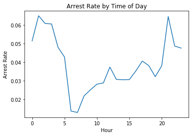

The arrest rate has a significant spike overnight, and then dips in the early morning hours.

## Are drug-related stops on the rise?

Plotting drug-related stops

In a small portion of traffic stops, drugs are found in the vehicle during a search. In this exercise, you’ll assess whether these drug-related stops are becoming more common over time.

The Boolean column drugs_related_stop indicates whether drugs were found during a given stop. We’ll calculate the annual drug rate by resampling this column, and then we’ll use a line plot to visualize how the rate has changed over time.

# Calculate the annual rate of drug-related stops
# Save the annual rate of drug-related stops
annual_drug_rate = ri.drugs_related_stop.resample("A").mean()
display(annual_drug_rate)

# Create a line plot of 'annual_drug_rate'
annual_drug_rate.plot()

# Display the plot
plt.show()

stop_date_time
2005-12-31    0.006501
2006-12-31    0.007258
2007-12-31    0.007970
2008-12-31    0.007505
2009-12-31    0.009889
2010-12-31    0.010081
2011-12-31    0.009731
2012-12-31    0.009921
2013-12-31    0.013094
2014-12-31    0.013826
2015-12-31    0.012266
Freq: A-DEC, Name: drugs_related_stop, dtype: float64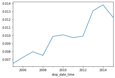

The rate of drug-related stops nearly doubled over the course of 10 years. Why might that be the case?

Comparing drug and search rates

The rate of drug-related stops increased significantly between 2005 and 2015. We might hypothesize that the rate of vehicle searches was also increasing, which would have led to an increase in drug-related stops even if more drivers were not carrying drugs.

We can test this hypothesis by calculating the annual search rate, and then plotting it against the annual drug rate. If the hypothesis is true, then we’ll see both rates increasing over time.

# Calculate and save the annual search rate
annual_search_rate = ri.search_conducted.resample("A").mean()

# Concatenate 'annual_drug_rate' and 'annual_search_rate'
annual = pd.concat([annual_drug_rate, annual_search_rate], axis="columns")

# Create subplots from 'annual'
annual.plot(subplots=True)

# Display the subplots
plt.show()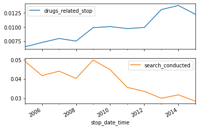

The rate of drug-related stops increased even though the search rate decreased, disproving our hypothesis.

What violations are caught in each district?

Tallying violations by district

The state of Rhode Island is broken into six police districts, also known as zones. How do the zones compare in terms of what violations are caught by police?

We’ll create a frequency table to determine how many violations of each type took place in each of the six zones. Then, we’ll filter the table to focus on the “K” zones, which we’ll examine further.

# Create a frequency table of districts and violations
# Save the frequency table as 'all_zones'
all_zones = pd.crosstab(ri.district, ri.violation)
display(all_zones)

# Select rows 'Zone K1' through 'Zone K3'
# Save the smaller table as 'k_zones'
k_zones = all_zones.loc["Zone K1":"Zone K3"]
k_zones

violation	Equipment	Moving violation	Other	Registration/plates	Seat belt	Speeding
district
Zone K1	672	1254	290	120	0	5960
Zone K2	2061	2962	942	768	481	10448
Zone K3	2302	2898	705	695	638	12322
Zone X1	296	671	143	38	74	1119
Zone X3	2049	3086	769	671	820	8779
Zone X4	3541	5353	1560	1411	843	9795

violation	Equipment	Moving violation	Other	Registration/plates	Seat belt	Speeding
district
Zone K1	672	1254	290	120	0	5960
Zone K2	2061	2962	942	768	481	10448
Zone K3	2302	2898	705	695	638	12322

We’ll plot the violations so that you can compare these districts.

Plotting violations by district

Now that we’ve created a frequency table focused on the “K” zones, we’ll visualize the data to help us compare what violations are being caught in each zone.

First we’ll create a bar plot, which is an appropriate plot type since we’re comparing categorical data. Then we’ll create a stacked bar plot in order to get a slightly different look at the data.

# Create a bar plot of 'k_zones'
k_zones.plot(kind="bar")

# Display the plot
plt.show()

# Create a stacked bar plot of 'k_zones'
k_zones.plot(kind="bar", stacked=True)

# Display the plot
plt.show()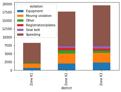

The vast majority of traffic stops in Zone K1 are for speeding, and Zones K2 and K3 are remarkably similar to one another in terms of violations.

How long might you be stopped for a violation?

Converting stop durations to numbers

In the traffic stops dataset, the stop_duration column tells us approximately how long the driver was detained by the officer. Unfortunately, the durations are stored as strings, such as '0-15 Min'. How can we make this data easier to analyze?

We’ll convert the stop durations to integers. Because the precise durations are not available, we’ll have to estimate the numbers using reasonable values:

Convert '0-15 Min' to 8
Convert '16-30 Min' to 23
Convert '30+ Min' to 45

# Create a dictionary that maps strings to integers
mapping = {"0-15 Min":8, '16-30 Min':23, '30+ Min':45}

# Convert the 'stop_duration' strings to integers using the 'mapping'
ri['stop_minutes'] = ri.stop_duration.map(mapping)

# Print the unique values in 'stop_minutes'
ri.stop_minutes.unique()

array([ 8, 23, 45], dtype=int64)

Next we’ll analyze the stop length for each type of violation.

Plotting stop length

If you were stopped for a particular violation, how long might you expect to be detained?

We’ll visualize the average length of time drivers are stopped for each type of violation. Rather than using the violation column we’ll use violation_raw since it contains more detailed descriptions of the violations.

# Calculate the mean 'stop_minutes' for each value in 'violation_raw'
# Save the resulting Series as 'stop_length'
stop_length = ri.groupby("violation_raw").stop_minutes.mean()
display(stop_length)

# Sort 'stop_length' by its values and create a horizontal bar plot
stop_length.sort_values().plot(kind="barh")

# Display the plot
plt.show()

violation_raw
APB                                 17.967033
Call for Service                    22.124371
Equipment/Inspection Violation      11.445655
Motorist Assist/Courtesy            17.741463
Other Traffic Violation             13.844490
Registration Violation              13.736970
Seatbelt Violation                   9.662815
Special Detail/Directed Patrol      15.123632
Speeding                            10.581562
Suspicious Person                   14.910714
Violation of City/Town Ordinance    13.254144
Warrant                             24.055556
Name: stop_minutes, dtype: float64

Analyzing the effect of weather on policing

We will use a second dataset to explore the impact of weather conditions on police behavior during traffic stops. We will be merging and reshaping datasets, assessing whether a data source is trustworthy, working with categorical data, and other advanced skills.

Exploring the weather dataset

Plotting the temperature

We’ll examine the temperature columns from the weather dataset to assess whether the data seems trustworthy. First we’ll print the summary statistics, and then you’ll visualize the data using a box plot.

# Read 'weather.csv' into a DataFrame named 'weather'
weather = pd.read_csv("../datasets/weather.csv")
display(weather.head())

# Describe the temperature columns
display(weather[["TMIN", "TAVG", "TMAX"]].describe().T)

# Create a box plot of the temperature columns
weather[["TMIN", "TAVG", "TMAX"]].plot(kind='box')

# Display the plot
plt.show()

	STATION	DATE	TAVG	TMIN	TMAX	AWND	WSF2	WT01	WT02	WT03	...	WT11	WT13	WT14	WT15	WT16	WT17	WT18	WT19	WT21	WT22
0	USW00014765	2005-01-01	44.0	35	53	8.95	25.1	1.0	NaN	NaN	...	NaN	1.0	NaN	NaN	NaN	NaN	NaN	NaN	NaN	NaN
1	USW00014765	2005-01-02	36.0	28	44	9.40	14.1	NaN	NaN	NaN	...	NaN	NaN	NaN	NaN	1.0	NaN	1.0	NaN	NaN	NaN
2	USW00014765	2005-01-03	49.0	44	53	6.93	17.0	1.0	NaN	NaN	...	NaN	1.0	NaN	NaN	1.0	NaN	NaN	NaN	NaN	NaN
3	USW00014765	2005-01-04	42.0	39	45	6.93	16.1	1.0	NaN	NaN	...	NaN	1.0	1.0	NaN	1.0	NaN	NaN	NaN	NaN	NaN
4	USW00014765	2005-01-05	36.0	28	43	7.83	17.0	1.0	NaN	NaN	...	NaN	1.0	NaN	NaN	1.0	NaN	1.0	NaN	NaN	NaN

5 rows × 27 columns

	count	mean	std	min	25%	50%	75%	max
TMIN	4017.0	43.484441	17.020298	-5.0	30.0	44.0	58.0	77.0
TAVG	1217.0	52.493016	17.830714	6.0	39.0	54.0	68.0	86.0
TMAX	4017.0	61.268608	18.199517	15.0	47.0	62.0	77.0	102.0

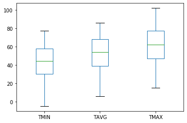
The temperature data looks good so far: the TAVG values are in between TMIN and TMAX, and the measurements and ranges seem reasonable.

### Plotting the temperature difference

We’ll continue to assess whether the dataset seems trustworthy by plotting the difference between the maximum and minimum temperatures.

# Create a 'TDIFF' column that represents temperature difference
weather["TDIFF"] = weather.TMAX - weather.TMIN

# Describe the 'TDIFF' column
display(weather.TDIFF.describe())

# Create a histogram with 20 bins to visualize 'TDIFF'
weather.TDIFF.plot(kind="hist", bins=20)

# Display the plot
plt.show()

count    4017.000000
mean       17.784167
std         6.350720
min         2.000000
25%        14.000000
50%        18.000000
75%        22.000000
max        43.000000
Name: TDIFF, dtype: float64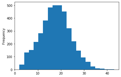

The TDIFF column has no negative values and its distribution is approximately normal, both of which are signs that the data is trustworthy.

Categorizing the weather

Counting bad weather conditions

The weather DataFrame contains 20 columns that start with 'WT', each of which represents a bad weather condition. For example:

WT05 indicates “Hail”
WT11 indicates “High or damaging winds”
WT17 indicates “Freezing rain”

For every row in the dataset, each WT column contains either a 1 (meaning the condition was present that day) or NaN (meaning the condition was not present).

We’ll quantify “how bad” the weather was each day by counting the number of 1 values in each row.

# Copy 'WT01' through 'WT22' to a new DataFrame
WT = weather.loc[:, "WT01":"WT22"]

# Calculate the sum of each row in 'WT'
weather['bad_conditions'] = WT.sum(axis="columns")

# Replace missing values in 'bad_conditions' with '0'
weather['bad_conditions'] = weather.bad_conditions.fillna(0).astype('int')

# Create a histogram to visualize 'bad_conditions'
weather.bad_conditions.plot(kind="hist")

# Display the plot
plt.show()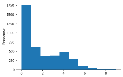

It looks like many days didn’t have any bad weather conditions, and only a small portion of days had more than four bad weather conditions.

Rating the weather conditions

We counted the number of bad weather conditions each day. We’ll use the counts to create a rating system for the weather.

The counts range from 0 to 9, and should be converted to ratings as follows:

Convert 0 to ‘good’
Convert 1 through 4 to ‘bad’
Convert 5 through 9 to ‘worse’

# Count the unique values in 'bad_conditions' and sort the index
display(weather.bad_conditions.value_counts().sort_index())

# Create a dictionary that maps integers to strings
mapping = {0:'good', 1:'bad', 2:'bad', 3:'bad', 4:'bad', 5:'worse', 6:'worse', 7:'worse', 8:'worse', 9:'worse'}

# Convert the 'bad_conditions' integers to strings using the 'mapping'
weather['rating'] = weather.bad_conditions.map(mapping)

# Count the unique values in 'rating'
weather.rating.value_counts()

0    1749
1     613
2     367
3     380
4     476
5     282
6     101
7      41
8       4
9       4
Name: bad_conditions, dtype: int64

bad      1836
good     1749
worse     432
Name: rating, dtype: int64

Changing the data type to category

Since the rating column only has a few possible values, we’ll change its data type to category in order to store the data more efficiently. we’ll also specify a logical order for the categories, which will be useful for future work.

# Create a list of weather ratings in logical order
cats = ['good', 'bad', 'worse']
# Change the data type of 'rating' to category
weather['rating'] = weather.rating.astype(CategoricalDtype(ordered=True, categories=cats))

# Examine the head of 'rating'
weather.rating.head()

0    bad
1    bad
2    bad
3    bad
4    bad
Name: rating, dtype: category
Categories (3, object): [good < bad < worse]

We’ll use the rating column in future exercises to analyze the effects of weather on police behavior.

Merging datasets

Preparing the DataFrames

We’ll prepare the traffic stop and weather rating DataFrames so that they’re ready to be merged:

With the ri DataFrame, we’ll move the stop_datetime index to a column since the index will be lost during the merge.
With the weather DataFrame, we’ll select the DATE and rating columns and put them in a new DataFrame.

# Reset the index of 'ri'
ri.reset_index(inplace=True)

# Examine the head of 'ri'
display(ri.head())

# Create a DataFrame from the 'DATE' and 'rating' columns
weather_rating = weather[["DATE", "rating"]]

# Examine the head of 'weather_rating'
weather_rating.head()

	stop_date_time	stop_date	stop_time	driver_gender	driver_race	violation_raw	violation	search_conducted	search_type	stop_outcome	is_arrested	stop_duration	drugs_related_stop	district	frisk	stop_minutes
0	2005-01-04 12:55:00	2005-01-04	12:55	M	White	Equipment/Inspection Violation	Equipment	False	NaN	Citation	False	0-15 Min	False	Zone X4	False	8
1	2005-01-23 23:15:00	2005-01-23	23:15	M	White	Speeding	Speeding	False	NaN	Citation	False	0-15 Min	False	Zone K3	False	8
2	2005-02-17 04:15:00	2005-02-17	04:15	M	White	Speeding	Speeding	False	NaN	Citation	False	0-15 Min	False	Zone X4	False	8
3	2005-02-20 17:15:00	2005-02-20	17:15	M	White	Call for Service	Other	False	NaN	Arrest Driver	True	16-30 Min	False	Zone X1	False	23
4	2005-02-24 01:20:00	2005-02-24	01:20	F	White	Speeding	Speeding	False	NaN	Citation	False	0-15 Min	False	Zone X3	False	8

	DATE	rating
0	2005-01-01	bad
1	2005-01-02	bad
2	2005-01-03	bad
3	2005-01-04	bad
4	2005-01-05	bad

The ri and weather_rating DataFrames are now ready to be merged.

Merging the DataFrames

We’ll merge the ri and weather_rating DataFrames into a new DataFrame, ri_weather.

The DataFrames will be joined using the stop_date column from ri and the DATE column from weather_rating. Thankfully the date formatting matches exactly, which is not always the case!

Once the merge is complete, we’ll set stop_datetime as the index

# Examine the shape of 'ri'
print(ri.shape)

# Merge 'ri' and 'weather_rating' using a left join
ri_weather = pd.merge(left=ri, right=weather_rating, left_on='stop_date', right_on='DATE', how='left')

# Examine the shape of 'ri_weather'
print(ri_weather.shape)

# Set 'stop_datetime' as the index of 'ri_weather'
ri_weather.set_index('stop_date_time', inplace=True)
ri_weather.head()

(86536, 16)
(86536, 18)

	stop_date	stop_time	driver_gender	driver_race	violation_raw	violation	search_conducted	search_type	stop_outcome	is_arrested	stop_duration	drugs_related_stop	district	frisk	stop_minutes	DATE	rating
stop_date_time
2005-01-04 12:55:00	2005-01-04	12:55	M	White	Equipment/Inspection Violation	Equipment	False	NaN	Citation	False	0-15 Min	False	Zone X4	False	8	2005-01-04	bad
2005-01-23 23:15:00	2005-01-23	23:15	M	White	Speeding	Speeding	False	NaN	Citation	False	0-15 Min	False	Zone K3	False	8	2005-01-23	worse
2005-02-17 04:15:00	2005-02-17	04:15	M	White	Speeding	Speeding	False	NaN	Citation	False	0-15 Min	False	Zone X4	False	8	2005-02-17	good
2005-02-20 17:15:00	2005-02-20	17:15	M	White	Call for Service	Other	False	NaN	Arrest Driver	True	16-30 Min	False	Zone X1	False	23	2005-02-20	bad
2005-02-24 01:20:00	2005-02-24	01:20	F	White	Speeding	Speeding	False	NaN	Citation	False	0-15 Min	False	Zone X3	False	8	2005-02-24	bad

We’ll use ri_weather to analyze the relationship between weather conditions and police behavior.

Does weather affect the arrest rate?

Comparing arrest rates by weather rating

Do police officers arrest drivers more often when the weather is bad? Let’s find out below!

First, we’ll calculate the overall arrest rate.
Then, we’ll calculate the arrest rate for each of the weather ratings we previously assigned.
Finally, we’ll add violation type as a second factor in the analysis, to see if that accounts for any differences in the arrest rate.

Since we previously defined a logical order for the weather categories, good < bad < worse, they will be sorted that way in the results.

# Calculate the overall arrest rate
print(ri_weather.is_arrested.mean())

0.0355690117407784

# Calculate the arrest rate for each 'rating'
ri_weather.groupby("rating").is_arrested.mean()

rating
good     0.033715
bad      0.036261
worse    0.041667
Name: is_arrested, dtype: float64

# Calculate the arrest rate for each 'violation' and 'rating'
ri_weather.groupby(["violation", 'rating']).is_arrested.mean()

violation            rating
Equipment            good      0.059007
                     bad       0.066311
                     worse     0.097357
Moving violation     good      0.056227
                     bad       0.058050
                     worse     0.065860
Other                good      0.076966
                     bad       0.087443
                     worse     0.062893
Registration/plates  good      0.081574
                     bad       0.098160
                     worse     0.115625
Seat belt            good      0.028587
                     bad       0.022493
                     worse     0.000000
Speeding             good      0.013405
                     bad       0.013314
                     worse     0.016886
Name: is_arrested, dtype: float64

The arrest rate increases as the weather gets worse, and that trend persists across many of the violation types. This doesn’t prove a causal link, but it’s quite an interesting result!

Selecting from a multi-indexed Series

The output of a single .groupby() operation on multiple columns is a Series with a MultiIndex. Working with this type of object is similar to working with a DataFrame:

The outer index level is like the DataFrame rows.
The inner index level is like the DataFrame columns.

# Save the output of the groupby operation from the last exercise
arrest_rate = ri_weather.groupby(['violation', 'rating']).is_arrested.mean()


# Print the arrest rate for moving violations in bad weather
display(arrest_rate.loc["Moving violation", "bad"])

# Print the arrest rates for speeding violations in all three weather conditions
arrest_rate.loc["Speeding"]

0.05804964058049641

rating
good     0.013405
bad      0.013314
worse    0.016886
Name: is_arrested, dtype: float64

Reshaping the arrest rate data

We’ll start by reshaping the arrest_rate Series into a DataFrame. This is a useful step when working with any multi-indexed Series, since it enables you to access the full range of DataFrame methods.

Then, we’ll create the exact same DataFrame using a pivot table. This is a great example of how pandas often gives you more than one way to reach the same result!

# Unstack the 'arrest_rate' Series into a DataFrame
display(arrest_rate.unstack())

# Create the same DataFrame using a pivot table
ri_weather.pivot_table(index='violation', columns='rating', values='is_arrested')

rating	good	bad	worse
violation
Equipment	0.059007	0.066311	0.097357
Moving violation	0.056227	0.058050	0.065860
Other	0.076966	0.087443	0.062893
Registration/plates	0.081574	0.098160	0.115625
Seat belt	0.028587	0.022493	0.000000
Speeding	0.013405	0.013314	0.016886

rating	good	bad	worse
violation
Equipment	0.059007	0.066311	0.097357
Moving violation	0.056227	0.058050	0.065860
Other	0.076966	0.087443	0.062893
Registration/plates	0.081574	0.098160	0.115625
Seat belt	0.028587	0.022493	0.000000
Speeding	0.013405	0.013314	0.016886